Lab Objective

In this lab we set up and used our simulator environment for localization.

Prelab

I didn’t run into any unexpected issues setting up the simulator, except I had to install missing graphics packages into my WSL environment since I’m on Windows 11. I also discovered that VSCode’s Jupyter Notebook is different from Jupyter Lab.

Open-loop control

I programmed the robot to move in a square pattern using the set_vel command. The robot moves forward for a second, turns for a second, and repeats.

# reset / initialize
cmdr.reset_plotter()
cmdr.reset_sim()
init_time = time.time()
# loop forever (or until manual stop)
while cmdr.sim_is_running() and cmdr.plotter_is_running():
    # plot pose
    pose, gt_pose = cmdr.get_pose()
    cmdr.plot_odom(pose[0], pose[1])
    cmdr.plot_gt(gt_pose[0], gt_pose[1])
    # decide whether to rotate or move forward based on elapsed time
    t = time.time() - init_time
    t_mod = (t + 0.5) % 2
    if (t_mod <= 1):
        cmdr.set_vel(1,0) # forward
    else:
        cmdr.set_vel(0,1.52) # rotate

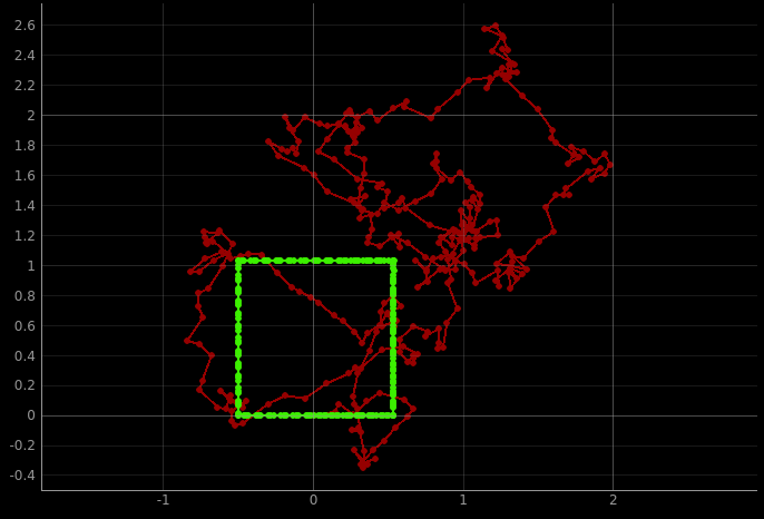
Ground truth position in green, odometry in red:

The robot doesn’t always execute the exact same shape, and will eventually drift and run into obstacles, because the robot speed and angular velocity can vary randomly.

Closed-loop control

I added random movement and obstacle avoidance with this code. The get_sensor command tells me the distance to the wall in front of the robot, which I can use to decide whether to turn or go forward.

# reset / initialize
cmdr.reset_plotter()
cmdr.reset_sim()
init_time = time.time()
rotation = 4
# loop forever (or until manual stop)
while cmdr.sim_is_running() and cmdr.plotter_is_running():
    # plot pose
    pose, gt_pose = cmdr.get_pose()
    cmdr.plot_odom(pose[0], pose[1])
    cmdr.plot_gt(gt_pose[0], gt_pose[1])
    # get sensor value (distance to wall in front)
    sensor_val = cmdr.get_sensor()[0]
    # decide whether to rotate or move forward based on sensor reading
    if (sensor_val >= 0.4):
        cmdr.set_vel(2,0) # forward
    else:
        cmdr.set_vel(0,rotation) # rotate
    if (np.random.rand() <= 0.01): # occasionally switch rotation direction
        rotation *= -1

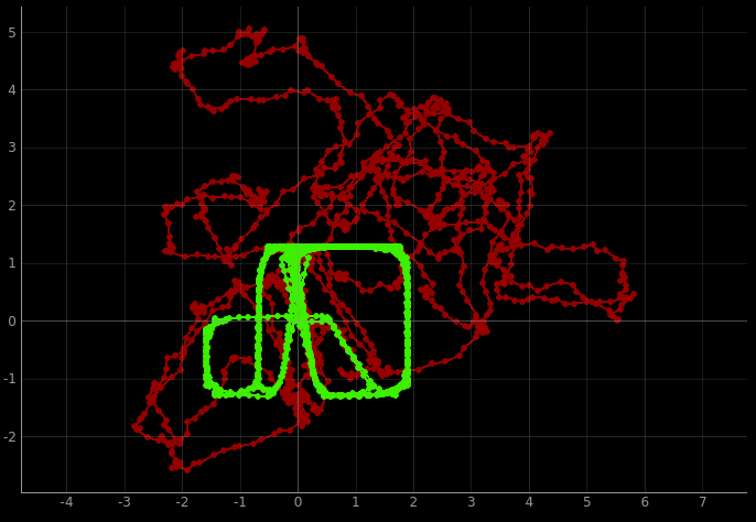
The robot successfully avoids obstacles while moving forward, and I could make it move pretty fast while doing so. However it still hits obstacles while rotating, because it has no way of knowing whether there’s a wall to the side of the robot.

Grid Localization

Implementing grid-based Bayes Filter localization in the sim invovled implementing some skeleton functions in the provided notebook.

My code is mostly based on Anya’s code from last year with some modifications and added comments explaining what’s going on.

Control

compute_control takes two poses (position and angle) and determines the control input u which would be necessary to go from one to the other. u represents a rotation-in-place, followed by a translation forward (since the simulated robot can only move forward on-axis), followed by another rotation-in-place.

def compute_control(cur_pose, prev_pose):
    delta_pose = (i - j for i, j in zip(cur_pose, prev_pose)) # = cur_pose - prev_pose
    dx, dy, dtheta = delta_pose
    angle = np.degrees(np.arctan2(dy, dx)) # angle of robot during translation
    prev_angle = prev_pose[2] # angle of robot before control
    # calculate control inputs
    delta_rot_1 = angle - prev_angle
    delta_trans = np.sqrt(dx**2 + dy**2)
    delta_rot_2 = dtheta - delta_rot_1 # this is because dtheta = delta_rot_1 + delta_rot_2
    return delta_rot_1, delta_trans, delta_rot_2

Motion Model

odom_motion_model computes the conditional probability \(P(x' \\| x, u)\), i.e. the probability of the robot being in the pose cur_pose given that it started in the pose prev_pose and the control input was u. This calculation relies on the assumption that control inputs have some known amount of noise which can be modeled as a Gaussian distribution.

def odom_motion_model(cur_pose, prev_pose, u):
    # find the control input which would be required to get to cur_pose from prev_pose
    x = compute_control(cur_pose, prev_pose)
    # find difference between this and the actual control input, u
    rot_1, trans, rot_2 = (i - j for i, j in zip(x, u))
    # normalize angles (into -180, 180 range)
    rot_1 = mapper.normalize_angle(rot_1)
    rot_2 = mapper.normalize_angle(rot_2)
    # calculate probabilities using gaussian, assuming certain noise levels in control
    prob_rot_1 = loc.gaussian(rot_1, 0, loc.odom_rot_sigma)
    prob_trans = loc.gaussian(trans, 0, loc.odom_trans_sigma)
    prob_rot_2 = loc.gaussian(rot_2, 0, loc.odom_rot_sigma)
    # combine probabilities (noise is independent, so just multiply)
    prob = prob_rot_1 * prob_trans * prob_rot_2
    return prob

Prediction Step

prediction_step updates \(\bar{bel}\) based on the motion model and the previous time step’s \(bel\).

This method is costly since it involves 6 nested for-loops. This could be made faster by parallelizing computations with numpy, but the other helper classes we were given don’t support this, and we can’t use numpy on the Arduino anyway, so I decided not to use numpy in this way.

As it is, the loop is made slightly faster by skipping contributions from cells which are very unlikely to be the actual previous position of the robot. This doesn’t lose any significant amount of precision because we are already discretizing the robot pose to a resolution of 1 foot and 20 degrees.

def prediction_step(cur_odom, prev_odom):
    # calculate control input
    u = compute_control(cur_odom, prev_odom)
    # initialize bel_bar array to zeros
    bel_bar = np.zeros((12, 9, 18))
    # loop through all cells for possible previous positions
    for cx_prev in range(12):
        for cy_prev in range(9):
            for ca_prev in range(18):
                # prior belief that we were in prev cell
                bel = loc.bel[cx_prev, cy_prev, ca_prev]
                # skip unlikely previous positions
                if (bel > 0.0001):
                    # convert from cell to world coords
                    prev_pose = mapper.from_map(cx_prev, cy_prev, ca_prev)
                    # loop through all possible current positions
                    for cx_cur in range(12):
                        for cy_cur in range(9):
                            for ca_cur in range(18):
                                # convert from cell to world coords
                                cur_pose = mapper.from_map(cx_cur, cy_cur, ca_cur)
                                # probability of moving from prev to cur cell
                                p = odom_motion_model(cur_pose, prev_pose, u)
                                # update bel_bar
                                bel_bar[cx_cur, cy_cur, ca_cur] += p * bel
    # normalize to sum to 1 to get a probability distribution
    loc.bel_bar = bel_bar/bel_bar.sum()

Sensor Model

To get from \(\bar{bel}\) to \(bel\) we need sensor data. sensor_model calculates \(P(z \\| x)\), the probability that a robot in some cell measured a distance of \(z\) (for each angle) given that the actual sensor readings for a robot in that cell would be \(x\).

We assume sensor noise follows a Gaussian distribution, so we just use loc.gaussian again.

def sensor_model(obs):
    return [loc.gaussian(loc.obs_range_data[i], obs[i], loc.sensor_sigma) for i in range(18)]

loc.gaussian explicitly supports parallel computation with numpy arrays, which means this method could be reduced to just return loc.gaussian(loc.obs_range_data, obs, loc.sensor_sigma), but this didn’t work for some reason.

Update Step

update_step combines bel_bar with the sensor conditional probability to get a final value for the probality of being in each cell.

def update_step():
    # loop through all possible current positions
    for cx_cur in range(12):
        for cy_cur in range(9):
            for ca_cur in range(18):
                # probability of being in cell (without accounting for sensor data)
                bel_bar = loc.bel_bar[cx_cur, cy_cur, ca_cur]
                # probability of being in cell given sensor readings
                p = sensor_model(mapper.get_views(cx_cur, cy_cur, ca_cur))
                p_mul = np.prod(p) # (noise of each reading is independent, so we can just multiply)
                # combined probability
                loc.bel[cx_cur, cy_cur, ca_cur] = p_mul * bel_bar
    # normalize to get a probability distribution
    loc.bel /= np.sum(loc.bel)

Running the Simulator

I ran the robot through the pre-planned trajectory and plotted ground truth position (green), odometry predicted position (red), and Bayes Filter predicted position (blue).

The Bayes Filter is working as expected, since the estimated position is much closer to the actual position than just the odometry-based prediction.

The white and grey cells show the \(\bar{bel}\) probability distribution. These values are generally highest near the robot’s actual position, meaning that our probability distribution is centered near the right place.