Lab Objective

We’re adding an IMU (inertial measurement unit) to the robot so it can measure its orientation, powering the system with a battery so it can be detached from the computer, and attaching it to a remote-controlled car.

1. IMU Setup

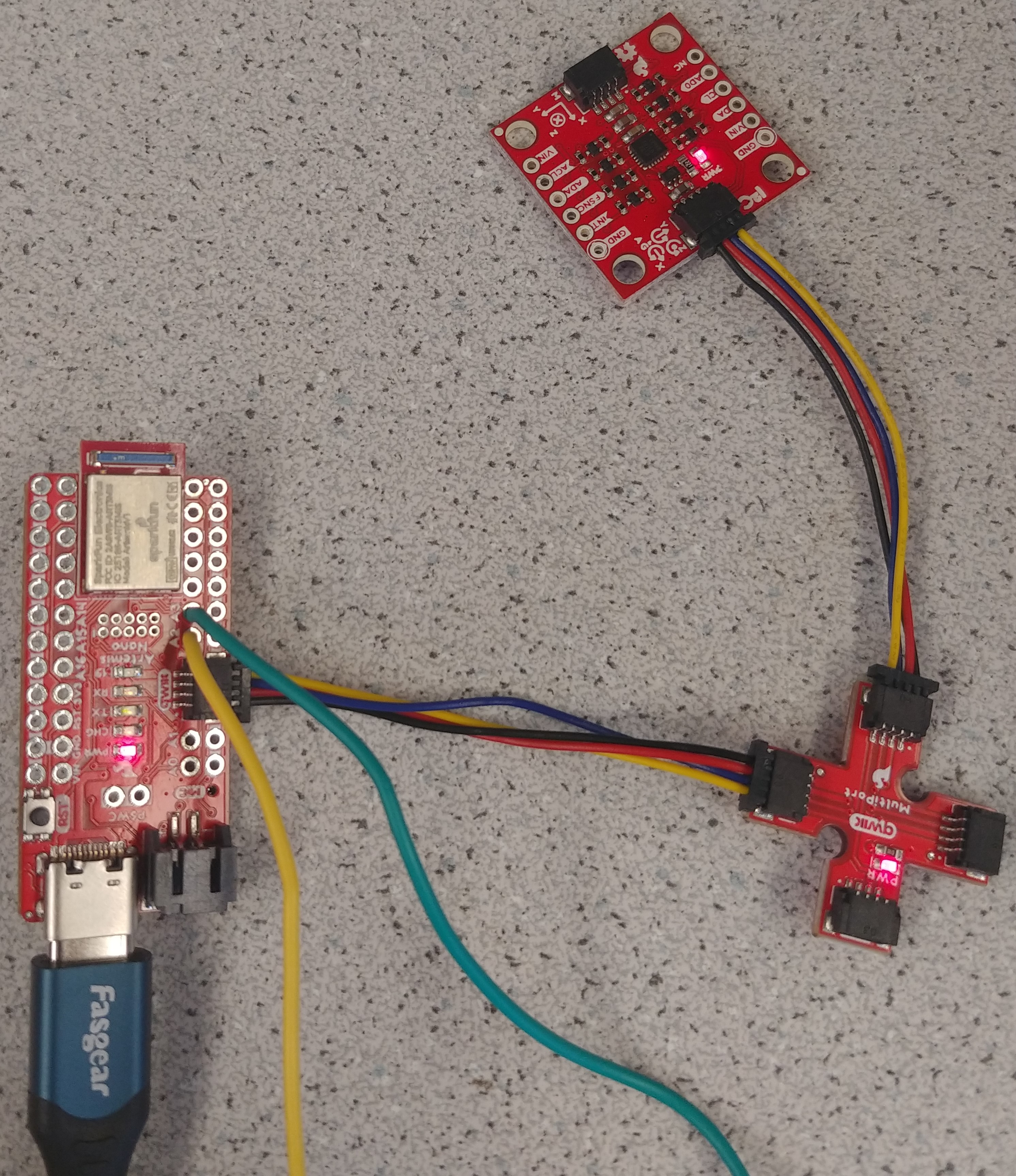
IMU attached to the Artemis over QWIIC:

Running the example code makes the board print accelerometer, gyroscope, and IMU temperature readings to the serial monitor:

In the code, AD0_VAL represents the last bit of the IMU’s I2C address. This is 0 by default, and changing it to 1 makes the code stop working:

This value should remain 0, unless we connect the ADR jumper, in which case it should be 1.

We can modify the code to print only the accelerometer data so that SerialPlot can display it:

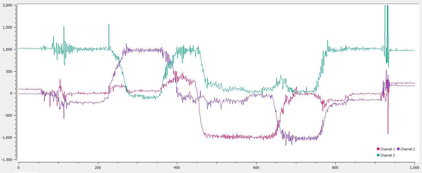
When holding the board flat parallel to the ground, the accelerometer measures about 0 mg in the x and y directions, and about 1000 mg in the z direction. If we rotate the board 90 degrees along the x or y axes, a different axis measures +/- 1000 mg.

If we print only the gyroscope data, we can see how moving around the IMU affects the gyroscope readings:

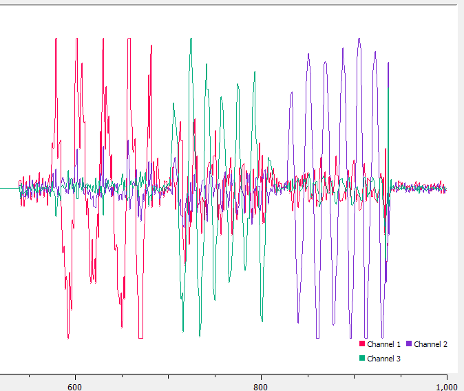
Rotating the board back and forth about its x axis produces an oscillation in the x channel (red). Rotating about the y axis produces an ocillation in the y channel (blue). Rotating about the z axis produces an oscillation in the z channel (green).

2. Accelerometer

I added the following code to loop() to calculate the roll and pitch of the IMU using accelerometer data:

I rotated the IMU around the faces of a wood block and recorded data in SerialPlot:

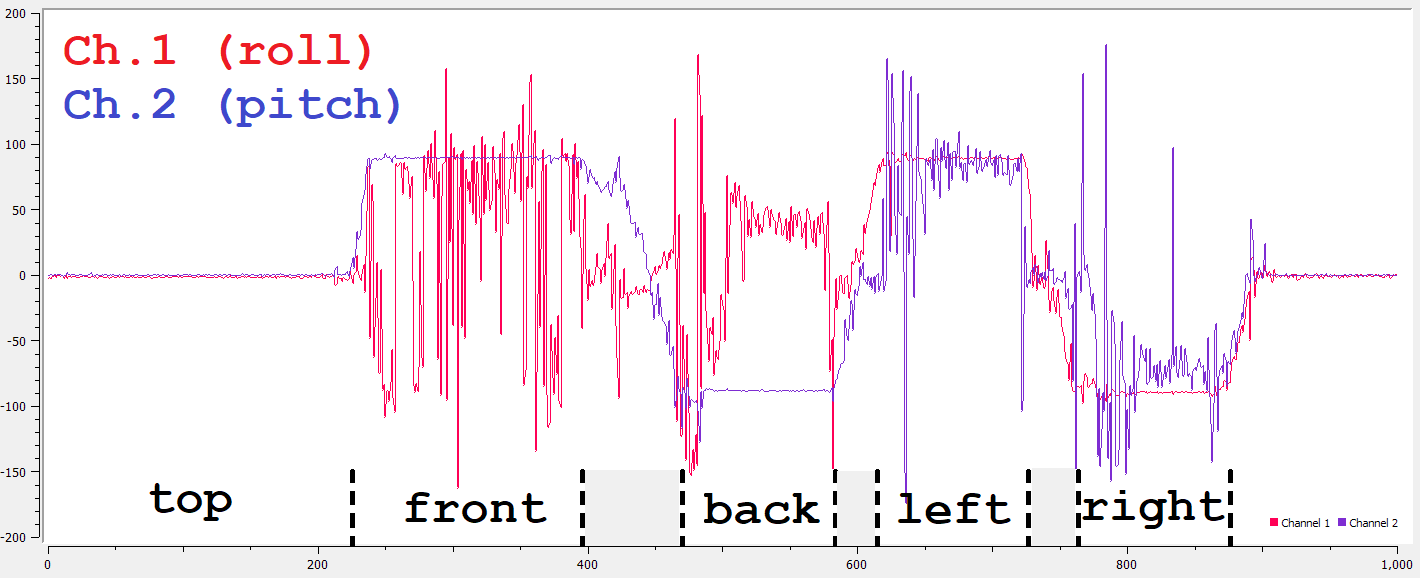
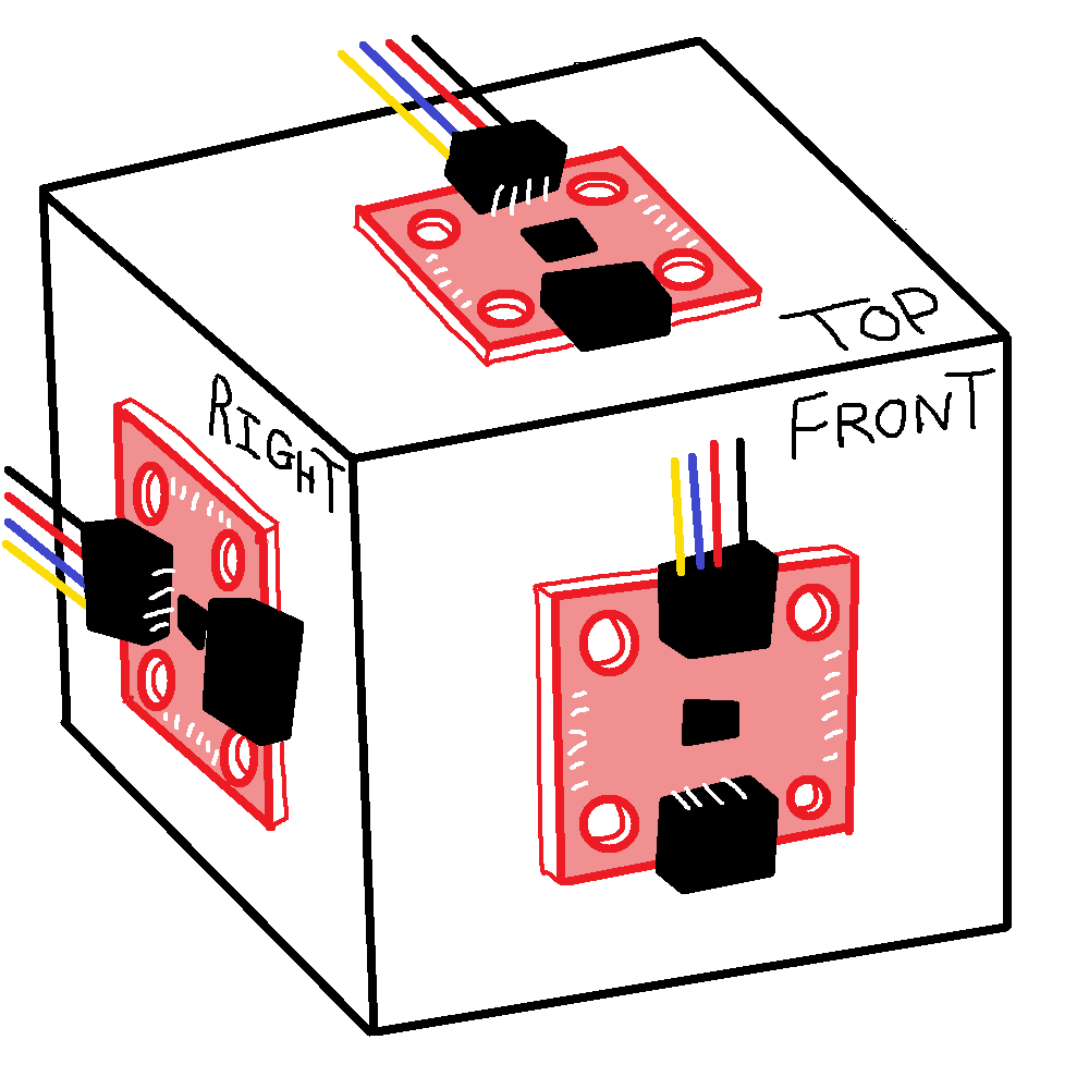
The expected vs. measured angles are summarized in this table. “Measured” values are averaged over each plateau in the graph.

Side	Pitch (expected)	Pitch (measured)	Roll (expected)	Roll (measured)
Top	0	0.34	0	-1.18
Front	90	89.74	?	31.63?
Back	-90	-87.90	?	25.59?
Left	?	78.96?	90	89.60
Right	?	-74.84?	-90	-89.53

I’ve put “?” where we can’t use this method to measure an angle, because atan2(y, x) is undefined when x and y are both 0. The especially spiky regions in the graph are caused by this problem.

Accuracy

Most of the measurements (which we can make using this method) are within 0.5 degrees of the expected values, except the pitch in the back position is 2.1 degrees off, and the roll in the top position is 1.2 degrees off.

These inaccuracies are small enough that they could be explained by the wood block not being a perfect rectangular prism, or by the table being angled slightly.

Noise

We can use a low-pass filter to remove sensor noise. To find a good cutoff frequency for the LPF, we first do a fast fourier transform (FFT) on some data. I recorded pitch/roll while moving the IMU moving in a “random” manner:

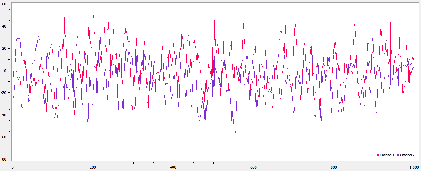
I exported this into a .csv file and found the Fourier transform of the roll data using Python:

import pandas as pd
import numpy as np
from scipy.fftpack import fft
import matplotlib.pyplot as plt

df = pd.read_csv('data.csv', sep=',', header=0)
time_data = df['Channel 1'].values
N = len(time_data) # number of samples
samples_per_sec = 31.0 # shown in SerialPlot
seconds = N/samples_per_sec # time elapsed between first and last samples
time = np.linspace(0, seconds, N) # time label for each sample (inferred)

freq_data = fft(time_data) # fast fourier transform
x = np.linspace(0, samples_per_sec*0.5, N//2) # x axis of FFT
y = 2/N * np.abs(freq_data[0:N//2]) # y axis of FFT

plt.plot(x, y) # then add labels, etc

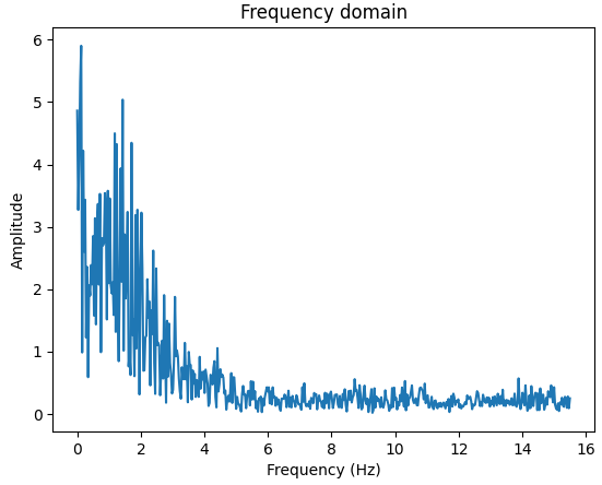
This graph is pretty noisy. So, I smoothed this data and plotted it again:

n = 15
y_smooth = np.convolve(y, np.ones(n)/(n), mode='same')

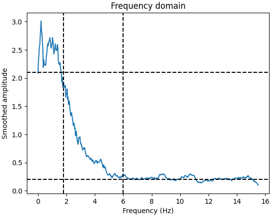
The frequency content is mostly below 5 Hz, and we can assume that everything above this is noise. So, the LPF cutoff frequency should be around 5 Hz.

To verify that we can use the same LPF parameters for both pitch and roll, I made this graph for pitch data using time_data = df['Channel 1'].values instead, and got a similar result:

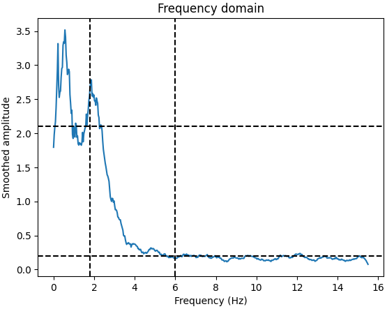
Assuming we get 31 samples/second, we have T=1/31, so using the formula alpha = T/(T + 1/(2πf)), we get that alpha should be 0.5. For testing purposes I set alpha to 0.25, so I could better see the effects of the filter.

The LPF is implemented in the Arduino sketch as follows:

// initialize variables before setup()
const float alpha = 0.25;
double pitch_a_LPF[] = {0, 0};
double roll_a_LPF[] = {0, 0};
// LPF code in loop():
pitch_a_LPF[1] = alpha*pitch_a + (1-alpha)*pitch_a_LPF[0];
pitch_a_LPF[0] = pitch_a_LPF[1];
roll_a_LPF[1] = alpha*roll_a + (1-alpha)*roll_a_LPF[0];
roll_a_LPF[0] = roll_a_LPF[1];

This successfully makes the output data less noisy.

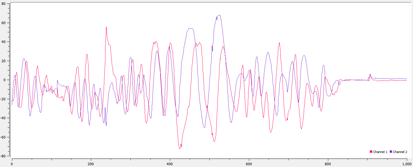
Choosing the cutoff frequency (or alpha) to be lower could get rid of more noise, but would also introduce more lag and could make the robot respond slower to sensor input.

3. Gyroscope

We can calculate pitch, roll, and yaw with gyroscope data using this Arduino code:

dt = (micros()-last_time)/1000000.; // time in seconds since last sample
last_time = micros();
pitch_g = pitch_g - myICM.gyrY()*dt;
roll_g = roll_g + myICM.gyrX()*dt;
yaw_g = yaw_g + myICM.gyrZ()*dt;
// then, print pitch_g, roll_g, yaw_g, pitch_a, and roll_a

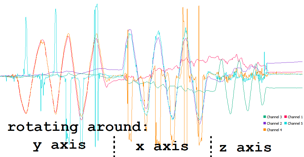
Both pitch measurements line up pretty well when the IMU is rotated around its y axis (pitch_g is red and pitch_a is orange). Similarly, roll_g (blue) and roll_a (teal) mostly agree when the IMU is rotated around its x axis. The green channel is yaw (z axis), but the accelerometer can’t measure yaw so there is nothing to compare to.

We can see the gyroscope measurements drift over time, because errors accumulate when we do integration.

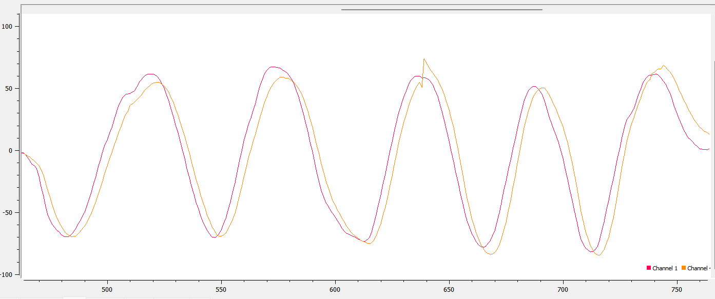
If we print the low-pass filtered accelerometer pitch and the gyroscope pitch, we can see that the LPF data lags behind compared to the gyroscope data:

Complimentary Filter

The drift and noise problems can both be solved with a complimentary filter:

// before setup():
float beta = 0.1 
// in loop():
pitch = (pitch - myICM.gyrY()*dt)*(1-beta) + pitch_a*beta;
roll = (roll + myICM.gyrX()*dt)*(1-beta) + roll_a*beta;

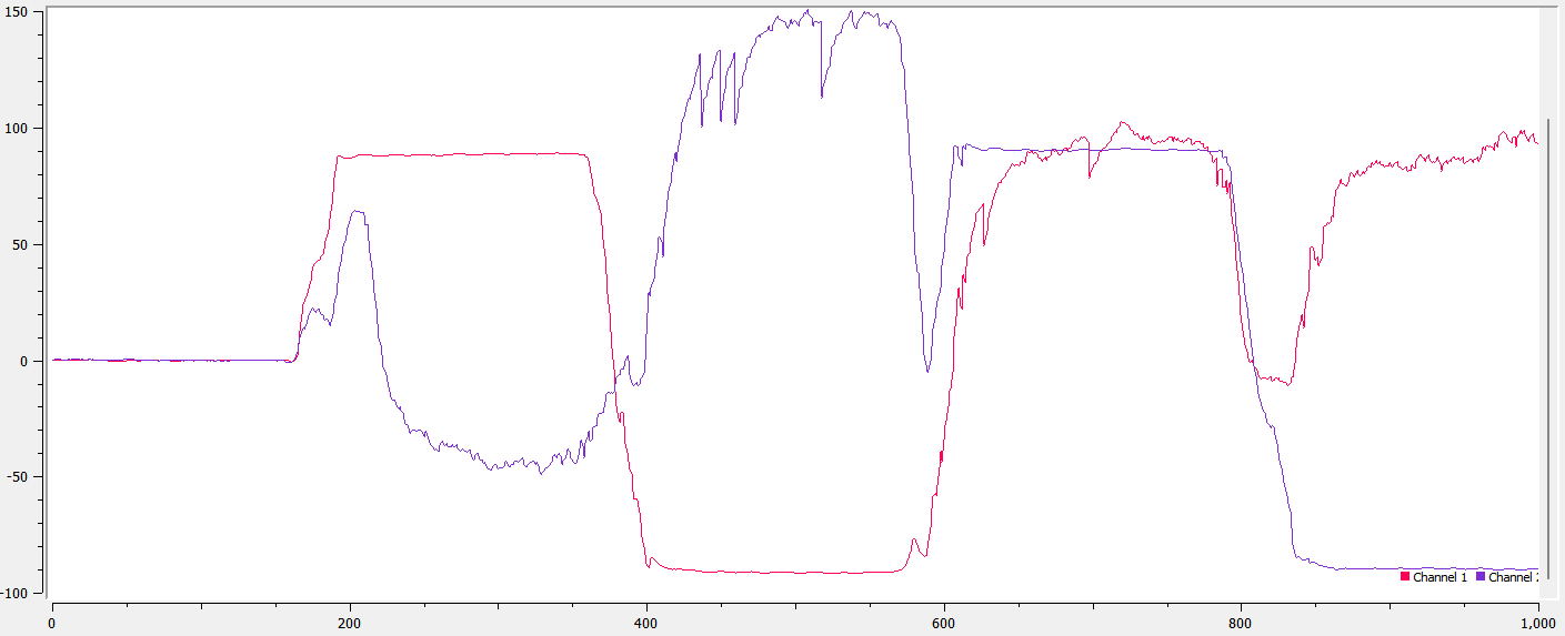
This gets rid of the drift of the gyroscope data, and gets rid of the noise of the accelerometer data. The result is accurate and stable. Each angle can be measured accurately at -90, 0, and 90 degrees, as shown above, where the IMU was placed against 5 sides of a block as before.

Setting beta to a higher value places more weight on the accelerometer measurements, and setting it lower places more weight on the gyroscope measurements. A value of beta=0.1 seems to work well.

4. Faster Sampling

To make the loop faster, I commented out all the print statements. I store the first 1000 data points in an array, and then print the time between the first and last samples:

// at the end of loop() after calculating pitch and roll:
if(n<1000) {
    T_array[n] = millis()/1000.0;
    pitch_array[n] = pitch;
    roll_array[n] = roll;
    n = n+1;
} else {
    Serial.println(T_array[999]-T_array[0]);
}

This printed 1.95, meaning the IMU gathered 1000 samples in 1.95 seconds, or 513 samples per second. This is significantly better than the 31 samples/sec we were getting before.

Storing Data

Copying the code I had from the previous lab, I can now store data from both TOFs and the IMU:

// in loop():
if(distanceSensor1.checkForDataReady()) {
    if(n_TOF1 < array_size) {
        TOF1_times[n_TOF1] = millis()/1000.0;
        TOF1_array[n_TOF1] = distanceSensor1.getDistance();
        n_TOF1 = n_TOF1+1;
        distanceSensor1.clearInterrupt();
    }
}
// same for sensor 2, in its own array

Instead of trying to store everything in one big array I decided to have separate arrays for each TOF, each TOF’s timestamps, the pitch and roll values, and IMU timestamps, for a total of 7 arrays:

// before setup():
int n_IMU = 0; // number of elements in IMU_times, pitch_array, and roll_array
int n_TOF1 = 0; // number of elements in TOF1_times, TOF1_array
int n_TOF2 = 0; // number of elements in TOF2_times, TOF2_array
#define array_size 1000
float TOF1_times[array_size];
float TOF2_times[array_size];
float TOF1_array[array_size];
float TOF2_array[array_size];
float IMU_times[array_size];
float pitch_array[array_size];
float roll_array[array_size];

Since each sensor can be “ready” at a different time, doing it this way means we don’t have to synchronize adding values from different sensors to the same array.

Memory

If we print the time between the first and last samples for the TOFs, we see they capture 1000 samples in about 95 seconds, or about 10.6 samples/second:

// in loop():
if (n_TOF1 == array_size && n_TOF2 == array_size && n_IMU == array_size) {
    Serial.print("IMU time: ");
    Serial.println(IMU_times[array_size-1]-IMU_times[0]);
    Serial.print("TOF1 time: ");
    Serial.println(TOF1_times[array_size-1]-TOF1_times[0]);
    Serial.print("TOF2 time: ");
    Serial.println(TOF2_times[array_size-1]-TOF2_times[0]);
}

The IMU takes 8.7 seconds, or 115 samples/second, which is slower than the 513 samples/second we were getting before because the Artemis can’t read from the IMU and the TOFs at the same time.

If we were constantly reading from all the sensors, we could read 115 + 10.6 + 10.6 = 136 samples/second. Each float is 4 bytes, and we also need 2 bytes for each timestamp, so each second we need to record 115*(4+4+2) + 10.6*(4+2) + 10.6*(4+2) = 1280 bytes of data. If we assume the Artemis has 360kB of memory, then we can store about 4.7 minutes of data.

If we wanted more data, we could store samples as integers instead of floats, since ints are 2 bytes instead of 4, and our measurements aren’t so precise that we need floats to store them.

Bluetooth

We can now send this data over Bluetooth instead of the serial USB cable. To do this, I moved all this code into a new robot command in the Bluetooth lab code, and implemented it in a manner similar to the GET_RAPID_5S command.

case GET_5S_DATA:
    // initialize
    n_IMU = 0; n_TOF1 = 0; n_TOF2 = 0; last_time = micros(); pitch = 0; roll = 0;
    command_start_time = (int)millis();
    // loop for 5 seconds
    while((int)millis() - command_start_time < 5000) {
        if (myICM.dataReady() && n_IMU < array_size)
        {
            myICM.getAGMT();
            // ... do the same pitch and roll calculations as before...
            IMU_times[n_IMU] = millis();
            pitch_array[n_IMU] = pitch;
            roll_array[n_IMU] = roll;
            n_IMU = n_IMU+1;
        }
        if(distanceSensor1.checkForDataReady() && n_TOF1 < array_size) {
            // ... similar code with different arrays
            // ...
        }
        if(distanceSensor2.checkForDataReady() && n_TOF2 < array_size) {
            // ... similar code with different arrays
            // ...
        }
    }

We collect all the data in arrays which are initialized globally, and then send the data over Bluetooth in chunks of at least 120 bytes each:

// in case GET_5S_DATA:
    tx_estring_value.clear();
    tx_characteristic_string.writeValue("IMU data:");
    for(int i=0; i<n_IMU; i++) {
        int t = IMU_times[i] - command_start_time;
        pitch = pitch_array[i];
        roll = roll_array[i];
        tx_estring_value.append("|T:");
        tx_estring_value.append(t);
        tx_estring_value.append("|P:");
        tx_estring_value.append(pitch);
        tx_estring_value.append("|R:");
        tx_estring_value.append(roll);
        if(tx_estring_value.get_length() >= 120 || i == n_IMU-1) { // send it
            tx_characteristic_string.writeValue(tx_estring_value.c_str());
            tx_estring_value.clear();
        }
    }
    tx_characteristic_string.writeValue("|TOF1 data:");
    for(int i=0; i<n_TOF1; i++) {
        int t = TOF1_times[i] - command_start_time;
        int D1 = TOF1_array[i];
        // ... similar code as for IMU, to build estring and send it
        // ...
    }
    tx_characteristic_string.writeValue("|TOF2 data:");
    // ... same code as for TOF 1 ...
    // ...
    tx_characteristic_string.writeValue("|Done sending data.");

On the Python side, we store received data with a callback:

received_strings = []
def callback_fn(uuid, value):
    received_strings.append(ble.bytearray_to_string(value))
ble.start_notify(ble.uuid['RX_STRING'], callback_fn)
ble.send_command(CMD.GET_5S_DATA, "")

We then process the data:

tokens_array = []
for st in received_strings:
    lst = st.split("|") # separate tokens
    if st[0]=="|": lst = lst[1:] # ignore empty token
    tokens_array += lst # collect tokens in list

IMU_time=[]; pitch=[]; roll=[]; TOF1_time=[]; distance_1=[]; TOF2_time=[]; distance_2=[]
t = -1; p = -1
for token in tokens_array:
    if len(token) >= 2:
        prefix = token[:2]
        data = token[2:]
        if prefix == "T:":
            t = int(data)/1000
        elif prefix == "P:":
            p = float(data)
        elif prefix == "R:":
            IMU_time.append(t)
            pitch.append(p)
            roll.append(float(data))
        elif prefix == "1:":
            TOF1_time.append(t)
            distance_1.append(int(data))
        elif prefix == "2:":
            TOF2_time.append(t)
            distance_2.append(int(data))

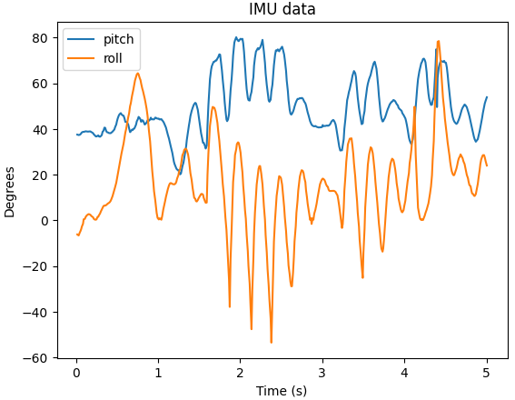
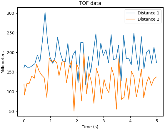
Then we print it with pyplot. These were the results when I shook the sensors around while sending the robot command:

5. Cut the Cord

To fully disconnect the robot from the computer, it needs to run off its own power supply.

We have three batteries, one 3.7V 850mAH battery and two 3.7V 650mAH ones. Since the motors consume more power than the Artemis, we will use the 850mAH battery to power the motors and motor drivers, so that the robot can operate for longer on a full charge.

I soldered one of the 650mAH batteries to a cable connector and attached it to the Artemis:

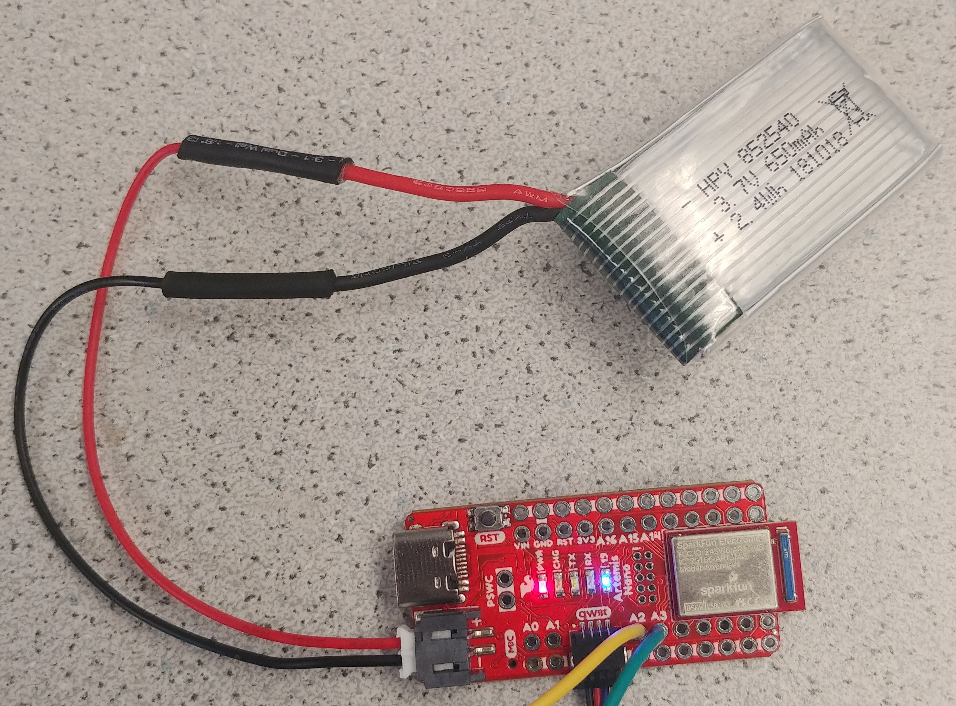
The LED I programmed to blink is blinking when the battery is plugged in, confirming that the board gets power. I can also receive Bluetooth data as before.

6. Record a Stunt

Controlling the RC car without any modifications:

The car generally moves and turns faster than I expected, and it’s hard to make it move/turn a small amount since it responds so quickly. Accelerating the car forward and sudddenly going backwards causes it to flip over, performing a kind of stunt.

Artemis and sensors attached to car:

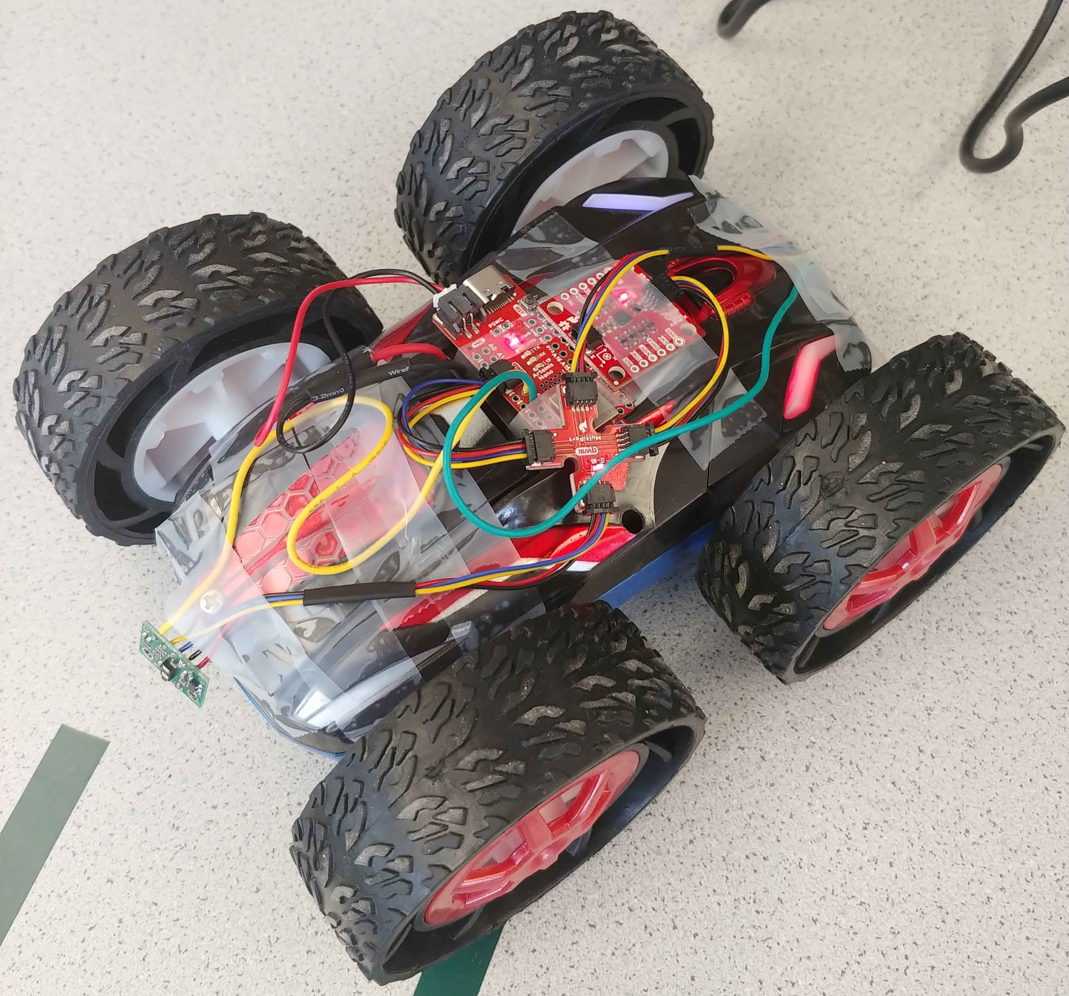
Controlling the RC car while recording TOF and IMU data:

Resulting 5 seconds of data:

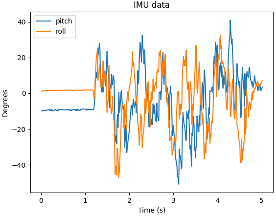
The pitch and roll calculations assume that the IMU’s acceleration is only caused by gravity, which is no longer true once the IMU is attached to a rapidly accelerating robot.

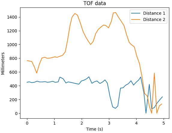
“Distance 1” is from the TOF sensor attached to the front, and “Distance 2” is from the TOF sensor attached to the back. We can see the spike in Distance 2 at 1.5 seconds when the robot starts moving. The dip in Distance 1 at 3 seconds is when the robot tilts forward once it starts moving in reverse, and the sensor detects the floor. At around 4 seconds both sensors give rapidly varying readings as the robot spins/hits the door. Everything past 5 seconds in the video isn’t recorded in the data.