Lab Objective

In this lab, I will be implementing a Kalman Filter to effectively speed up the slow time-of-flight sensor, allowing the robot to do the Lab 6 task (speeding towards a wall and stopping 1 foot away) faster.

System Model

The forces acting on the robot can be summarized as

\[\begin{align} F = u\cdot c - x'\cdot d = m \cdot x'' \end{align}\]

where \(u\) is the PWM control value, \(x\), \(x'\), and \(x''\) are position, velocity, and acceleration, and \(c\), \(d\), and \(m\) are unknown constants. We can rewrite this as

\[\begin{align} \begin{bmatrix} x' \\ x'' \end{bmatrix} = \begin{bmatrix} 0 & 1 \\ 0 & -d/m \end{bmatrix} \begin{bmatrix} x \\ x' \end{bmatrix} + \begin{bmatrix} 0 \\ c/m \end{bmatrix} u \end{align}\]

or,

\[\begin{align} \frac{d}{dt} \vec{x} = \mathbf{A} \vec{x} + \mathbf{B} u \end{align}\]

To get \(\mathbf{A}\) and \(\mathbf{B}\) we need \(d/m\) and \(c/m\), which we can get by solving the differential equation \(x'' + \frac{d}{m} x' = \frac{c}{m}u\).

Maximum Speed

If \(u\) is held constant at some value \(u_{\text{max}}\), then the robot stops accelerating once it hits its maximum speed. This means \(x' = x'_{\text{max}}\) and \(x'' = 0\). Plugging and solving gives us \(x'_{\text{max}} = u_{\text{max}}c/d\), or

\[\begin{align} d = \frac{u_{\text{max}}}{x'_{\text{max}}}c \end{align}\]

Ramping-up

If we solve the differential equation for \(x'\) with the initial condition that \(x'(t) = 0\), we get:

\[\begin{align} x'(t) = x'_{\text{max}} \cdot \left( 1 - e^{-d \cdot t/m} \right) \end{align}\]

This means that, if \(u\) is constant, the robot ramps up exponentially to its maximum speed. The robot is at 90% of its max speed when

\[\begin{align} 1 - e^{-d \cdot t/m} &= 0.9 \end{align}\]

Labeling this time-to-90% as \(t_{90}\) we can solve for \(m\):

\[\begin{align} m = -\frac{d\cdot t_{90}}{\ln(0.1)} \end{align}\]

Using these expressions for \(d\) and \(m\) we can solve for the unknown coefficients in \(\mathbf{A}\) and \(\mathbf{B}\):

\[\begin{align} \mathbf{A} &= \begin{bmatrix} 0 & 1 \\ 0 & \frac{\ln(0.1)}{t_{90}} \end{bmatrix}\\ \mathbf{B} &= \begin{bmatrix} 0 \\ -\frac{\ln(0.1)}{t_{90}}\cdot\frac{x'_{\text{max}}}{u_{\text{max}}} \end{bmatrix} \end{align}\]

Step Response

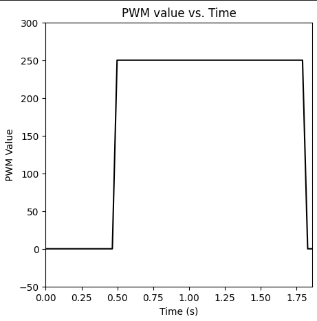
To measure \(x'_{\text{max}}\) and \(t_{90}\) I powered the robot with a step function and measured the response. I set the control PWM value to a constant \(u_\text{max} =\) 250, and powered it for 1.3 seconds, starting 3 meters away from a wall.

This was the PWM value over time:

The position and velocity are plotted below:

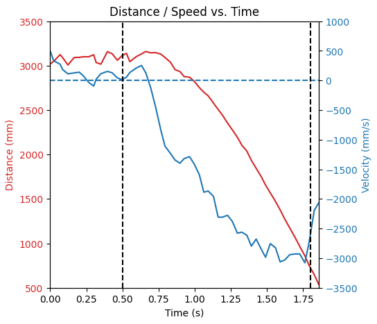
The robot reached a steady-state speed of 3 m/s briefly before crashing into the wall (this is the moment the data ends). So, we can say that \(x_{\text{max}} = 3000\) mm/s when \(u_{\text{max}} = 250\).

The time taken to reach 90% of the steady state speed, starting from 0 velocity, was around 0.9 seconds:

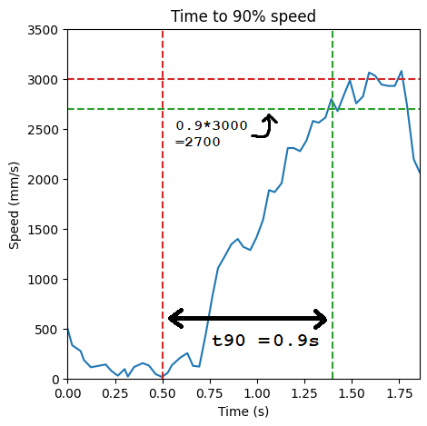
Based on these observations, I solved for the unknowns to get \(A_{2,2} = -2.56\) and \(B_{2,1} = 30.7\).

\(c\) is still unknown, but if we assume \(u_{\text{max}}c = 1\) newton, then we get a damping coefficient of \(d = 0.333\) Ns/m, and a mass of \(m = 0.130\) kg.

Kalman Filter

I modified this code written by Anya last year to get a Kalman filter:

# Initial state uncertainty 
sig = np.array([[5**2,0],[0,5**2]])

# A, B, C matrices
A = np.array([[0,1],[0,-2.56]])
B = np.array([[0],[30.7]])
C = np.array([[-1,0]])

# Process and sensor noise
sig_u = np.array([[10**2,0],[0,10**2]])
sig_z = np.array([[20**2]])

# Discretize A and B
delta_t = times[1] - times[0]
Ad = np.eye(2) + delta_t * A
Bd = delta_t * B

# Initial state
x = np.array([[-distancesMM[0]],[0]])

# KF estimation
def kf(x,u,sig,y):
    x_p = Ad.dot(x) + Bd.dot(u)                      # predicted state
    sig_p = Ad.dot(sig.dot(Ad.transpose())) + sig_u  # predicted state uncertainty
    
    y_m = y-C.dot(x_p)
    sig_m = C.dot(sig_p.dot(C.transpose())) + sig_z
    
    kf_gain = sig_p.dot(C.transpose().dot(np.linalg.inv(sig_m)))  # KF gain

    x_n   = x_p + kf_gain.dot(y_m)                   # new state 
    sig_n = (np.eye(2) - kf_gain.dot(C)).dot(sig_p)  # new state uncertainty

    return x_n, sig_n

I ran this code to test what the Kalman filter would output, and compared this to the raw measurements from my TOF sensor:

# Run code
kf_state = []
for u, d in zip(values, distancesMM):
    x, sig = kf(x, [[u/80]], sig, [[d]])
    kf_state.append(x[:,0])
# then plot kf_state...

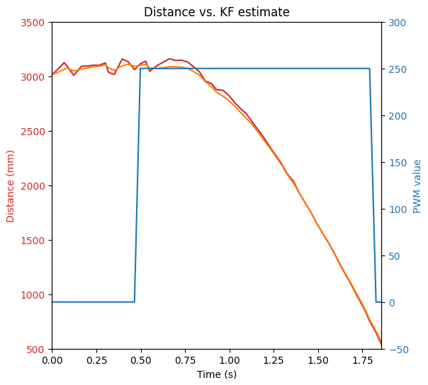
The Kalman filter successfully smooths out the sensor values and increases the number of “readings” we get.

Extrapolation

To increase the effective sampling speed of the TOF sensor without implementing a Kalman filter on the Arduino, I decided to use extrapolation to predict distance sensor readings based on the previous 2 actual readings.

To do this, I changed the code in my tof class:

int getDistanceEstimate() {
// update distance history if new data is available
if (sensor1.checkForDataReady()) {
    int newDist = distance1 * (1 - alpha) + alpha * sensor1.getDistance();
    sensor1.clearInterrupt();
    distance2 = distance1;
    distance1 = newDist;
    time2 = time1;
    time1 = millis();
    nPoints++;
}
if (nPoints >= 2) {
    // extrapolate from previous 2 points for estimate
    long time = millis();
    float slope = (float)(distance1 - distance2)/(time1 - time2);
    long timeDelta = time - time1;
    estimatedDistance = (int)(0.5 + distance1 + slope * timeDelta);
    return estimatedDistance;
} else {
    return distance1;
}
}

After adjusting the debug code to collect the raw distance data as well as the interpolated distance data, we can see that the interpolation successfully smooths out the slow sampling rate of the TOF:

(Raw distance in red, extrapolated distance in orange)

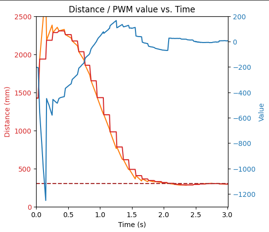
The PID controller works with these extrapolated distance values just as well: